Sign In
Sign In

Cloud Managed
MySQL

Ready-made clusters. No administration. With an hourly rate
Contact Sales
No Downtime
We provide 99.9% reliability according to SLA. We host servers exclusively in Tier IV data centers that meet all international security standards
Two-click Launch
Run the database directly in Hostman's modern control panel. All settings, services and facilities are available directly from the panel
Saving for Real
Use the database with hourly billing — and pay only for the services you use. No hidden charges and no imposed services
Convenient Scaling
Is the project growing? Connect additional resources. Hostman will provide as much power as your service requires

Pricing

MySQL
New York
1 x 3 GHz CPU
CPU
1 x 3 GHz
1 GB RAM
RAM
1 GB
20 GB NVMe
NVMe
20 GB
200 Mbps Bandwidth
Bandwidth
200 Mbps
$4
 /mo
2 x 3 GHz CPU
CPU
2 x 3 GHz
2 GB RAM
RAM
2 GB
60 GB NVMe
NVMe
60 GB
200 Mbps Bandwidth
Bandwidth
200 Mbps
$9
 /mo
2 x 3 GHz CPU
CPU
2 x 3 GHz
4 GB RAM
RAM
4 GB
80 GB NVMe
NVMe
80 GB
200 Mbps Bandwidth
Bandwidth
200 Mbps
$18
 /mo
4 x 3 GHz CPU
CPU
4 x 3 GHz
8 GB RAM
RAM
8 GB
160 GB NVMe
NVMe
160 GB
200 Mbps Bandwidth
Bandwidth
200 Mbps
$36
 /mo
6 x 3 GHz CPU
CPU
6 x 3 GHz
16 GB RAM
RAM
16 GB
320 GB NVMe
NVMe
320 GB
200 Mbps Bandwidth
Bandwidth
200 Mbps
$72
 /mo
8 x 3 GHz CPU
CPU
8 x 3 GHz
32 GB RAM
RAM
32 GB
640 GB NVMe
NVMe
640 GB
200 Mbps Bandwidth
Bandwidth
200 Mbps
$114
 /mo
16 x 3 GHz CPU
CPU
16 x 3 GHz
64 GB RAM
RAM
64 GB
1280 GB NVMe
NVMe
1280 GB
200 Mbps Bandwidth
Bandwidth
200 Mbps
$288
 /mo
Anup k.
Associate Cloud Engineer
5.0 out of 5

"Hostman Comprehensive Review of Simplicity and Potential"

It been few years that I have been working on Cloud and most of the cloud service...
Mansur H.
Security Researcher
5.0 out of 5

"A perfect fit for everything cloud services!"

Hostman's seemless integration, user-friendly interface and its robust features (backups, etc) makes it much easier...
Adedeji E.
DevOps Engineer
5.0 out of 5

"Superb User Experience"

For me, Hostman is exceptional because of it's flexibility and user-friendliness. The platform's ability to offer dedicated computing resources acr...
Yudhistira H.
Mid-Market(51-1000 emp.)
5.0 out of 5

"Streamlined Cloud Excellence!"

What I like best about Hostman is their exceptional speed of deployment, scalability, and robust security features. Their...
Mohammad Waqas S.
Biotechnologist and programmer
5.0 out of 5

"Seamless and easy to use Hosting Solution for Web Applications"

From the moment I signed up, the process has been seamless and straightforward...
Mohana R.
Senior Software Engineer
5.0 out of 5

"Availing Different DB Engine Services Provided by Hostman is Convenient for my Organization usecases"

Hostman manages the cloud operations...
Faizan A.
5.0 out of 5

"Hostman is a great fit for me"

Hostman is a great fit for me. What do you like best about Hostman? It was very easy to deploy my application and create database, I didn't have
Adam M.
5.0 out of 5

"Perfect website"

This website is extremely user friendly and easy to use. I had no problems so didn't have to contact customer support. Really good website and would recommend to others.
Anup K.
4.0 out of 5

"Simplifying Cloud Deployment with Strengths and Areas for Growth"

What I like best about Hostman is its unwavering commitment to simplicity...
Naila J.
5.0 out of 5

"Streamlined Deployment with Room for Improvement"

Hostman impresses with its user-friendly interface and seamless deployment process, simplifying web application hosting...

Trusted by 500+ companies and developers worldwide

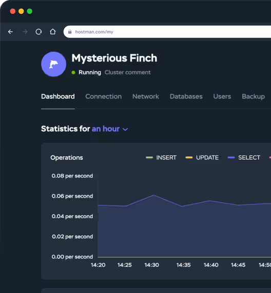
One panel to rule them all

Easily control your database, pricing plan, and additional services
through the intuitive Hostman management console
Easy set up and management
Ready-to-deploy cloud database solutions come pre-configured. Choose your setup, launch your database, and begin managing your data with ease
Saves time and resources
Forget about configuring hardware and software or manual database management—our service has it all covered for you
Security
Deploy databases on an isolated network to maintain private access solely through your own infrastructure

Everything is ready to deploy
your MySQL database to our
cloud — up and running
in seconds!

Databases for all tastes

MySQL

The most popular relational database management system from Oracle. Developed under an open-source model

PostgreSQL

An object-relational database management system. Supported by most UNIX platforms

Redis

A high-performance database that operates on a 'key-value model'. Often used for caching

MongoDB

A classic database management system oriented towards document storage and supporting JSON queries

OpenSearch

A system of search and analytics resources for monitoring applications and event logs

ClickHouse

A columnar analytical database. Supports queries to a large array of structured data in real-time mode

Kafka

An open-source messaging system. Known for its high speed and low latency

RabbitMQ

A messaging system based on the AMQP standard

Code locally, launch worldwide

Our servers, certified with ISO/IEC 27001, are located in Tier 3 data
centers across the US, Europe, and Asia
🇺🇸 San Francisco
🇺🇸 San Jose
🇺🇸 Texas
🇺🇸 New York
🇳🇱 Amsterdam
🇳🇬 Lagos
🇩🇪 Frankfurt
🇵🇱 Gdansk
🇦🇪 Dubai
🇸🇬 Singapore

Latest News

Python

Understanding HTTP Requests: Structure, Methods & Examples

HTTP is a key to communication on the internet. Methods of HTTP protocols allow clients to send requests to the servers and servers to send responses. Every website on the World Wide Web uses HTTP requests. So, it's necessary to understand them. This article explores the concept of HTTP requests, its structure, common methods, and real-life examples. This helps in understanding the functioning of the web.  What is an HTTP Request An HTTP request is a message where a client, such as a web browser, asks the host located on the server for a specific resource. Clients use URLs in HTTP requests which show the resources they want to access from the server.  Components of an HTTP Request Every HTTP request comprises three components namely; request line, headers and message body. Request Line  A request line is the start line in an HTTP request command. It is used to initialize an action on the server. A request line would also indicate what kind of method and version of HTTP protocol the client is using. Apart from the HTTP method, a request line also consists of a URI or URL to the path or protocol.  Request line example: GET /index.html HTTP/1.1 Headers Headers are right behind the request line. They offer client’s additional information to the server. Headers include data about the host, client’s user agent, language preferences and more. Server leverages this information to identify the browser and OS version of the client. HTTP request headers are case-sensitive, followed by a colon (:) and a value.  HTTP request Headers example:  Host: example.com User-Agent: Mozilla/5.0 (Windows NT 10.0; Win64; x64) AppleWebKit/537.36 (KHTML, like Gecko) Chrome/92.0.4515.107 Safari/537.36 Accept: application/json, text/plain, */* Accept-Language: en-US,en;q=0.9 Accept-Encoding: gzip, deflate, br Connection: keep-alive Message body The message body in an HTTP request is used to send data to the server. They are optional. So, not every HTTP request will have a message body. It depends on the HTTP request types the client uses. The HTTP requests that do have a message body, usually leverage POST to send information. Mainly, the server uses the message body to provide the requested data to the client.  Common HTTP Methods An HTTP request is a way to connect the client with the server. There can be many reasons for pursuing this connection. It might be to retrieve specific resources or delete certain information on the server. The most common HTTP request methods used daily include:  GET: To Retrieve Resources The biggest use case of an HTTP request is to ask the server for a specific set of data or resources. And that is done using the GET method. Every time a user wants to go to a website or any web page, the client browser first sends a request to retrieve the required data to load that page.  The GET in HTTP is a cacheable, safe, and idempotent method. However,, using a GET method multiple times can still impact server performance. The GET Method can only bring existing data from the server to the client. It can’t make any changes to it. So, the data or the resources would be in a read-only format.  POST: To Send Data When a client wants to retrieve any information, they use the GET method, but when providing some information to the server, the client uses the HTTP POST request. Let’s say users need to submit a form or upload a file. In this case, the client’s browser has to execute the POST method in HTTP to send the data to the server.  The message body in an HTTP request contains the data. When a client browser sends a POST request, the server processes the data. Using a POST method multiple times would result in the creation of different resources on the server.  PUT: To Update Resources Similar to the POST method, the PUT method also allows the client to add some information to the server. The only difference between both methods is that in POST, users submit new data whereas in PUT, they update the existing data.  When implementing the PUT request, the client has to specify the resource’s URL that it wants to update. The request also includes the updated representation of the resource in its message body. The server would simply replace the old representation with the new one.  The PUT method is idempotent so there is no harm in implementing multiple identical PUT requests as it would yield the same result.  DELETE: To Remove Resources As the name suggests, the DELETE method helps the client delete any specific resource from the server. Employing the DELETE request helps the client instruct the server to delete the resource mentioned in the request.  Upon the DELETE request of the client, when the server successfully deletes the specified resource, it sends back a confirmation to the client. Sending multiple identical DELETE requests would yield the same result.  What is an HTTP Response? When the server sends back a response to an HTTP request, it is called an HTTP response. The server acts upon the request it receives from the client browser. The HTTP response would then either consist of the requested resource or valuable information regarding the requested operation.  So, like an HTTP request, an HTTP response is also made up of three components with a slight difference. The response starts with a status line, and a request starts with a request line.  Status Line: As the request line does in an HTTP request, the status line in the HTTP response also indicates which version of HTTP is used along with the status code and the message specifying the outcome of the request.  Headers: Headers in the HTTP response offer additional information like the date and time of response, the type of content that is sent in the message body, details of the server and instructions on how to cache the content.  Body: The actual message or response data that the server sends to the client browser is placed in the message body. The content could be anything from XML, JSON or HTML for the web page, an image, or any other kind of requested resource. Status Codes and Their Meanings HTTP status codes represent the status of the client’s HTTP requests. They come as a part of an HTTP server response. Every status code consists of three digital numbers where the first digit of the code indicates the class or category of the response. There are five types of code groups. Status code group  Description  1xx Informational responses, continuing processing. 2xx Success responses, requests are processed, understood and accepted. 3xx Redirecting responses, suggests further action to complete the request. 4xx Error responses, show what’s wrong with the request on client-side. 5xx Error responses, state what went wrong with processing request on server-side. HTTP Headers and Their Importance HTTP headers provide additional information about requests and responses. This information is critical for communication between client and server. Headers are fundamental for web browsing and app functionality. They play an important role in the following web operations:  Host Identification Headers bear the identification of a server’s domain that is hosting the resources. It is helpful in scenarios where a server hosts multiple domains.  CachingHeaders like Expires and Cache-Control handle how browsers cache responses and intermediate proxies. It helps minimize loading time and server requests by determining how long a response needs to be stored.  Cookie ManagementHeaders like Set-Cookie and Cookie help save and send cookies respectively. They assist in tracking user behavior and maintain user sessions.  Security Headers also play a critical role in securing web applications. An Authorization header helps with user authentication whereas a Content-Security-Policy is used for mitigating XSS and other security risks.  Response ControlHeaders like Status inform whether the request was a success or a failure. It also provides the necessary details so the client can manage responses appropriately.  Practical Examples of HTTP Requests Here are a few real-life examples of how different HTTP requests are commonly used in day-to-day operations. All the examples are in Python with the use of the requests library. GET From entering a simple URL for the website to asking for a specific record from the web server, fetching data requires an HTTP GET request. Let’s say, the client wants to get the weather data of London. The implementation of GET requests in this use case would look like:  import requests response = requests.get("https://api.example.com/data", params={"param1": "value1", "param2": "value2"}) # Print the response print(response.status_code) print(response.json()) # Assuming the response is in JSON format POST When a user wants to create a new user in a hypothetical API. And wants to send the following JSON data: { "username": "newuser", "email": "[email protected]", "password": "securepassword" } The following Python code sends a POST request with the specified data: import requests url = "https://api.example.com/users" data = { "username": "newuser", "email": "[email protected]", "password": "securepassword" } # Make the POST request response = requests.post(url, json=data) if response.status_code == 201: print("User created successfully:", response.json()) else: print("Error:", response.status_code, response.text) PUT When a client wants to update the information of a user with a specific ID.  import requests url = "https://api.example.com/users/123" data = { "username": "updateduser", "email": "[email protected]" } # Make the PUT request response = requests.put(url, json=data) if response.status_code == 200: print("User updated successfully:", response.json()) else: print("Error:", response.status_code, response.text) DELETE When a client wants to delete a specific user. Here’s how it will look like in Python. import requests url = "https://api.example.com/users/123" # Make the DELETE request response = requests.delete(url) if response.status_code == 204: print("User deleted successfully.") else: print("Error:", response.status_code, response.text) Conclusion HTTP requests play a critical role in web interactions. Hence, it is essential to understand various request methods and how they work. However, the key to seamless communication lies in picking a suitable method. This also enhances the efficiency of web applications.  
04 October 2024 · 9 min to read
Python

How to Read Excel Files in Python using Pandas

Excel files are commonly used to organize, sort, and analyze data in a tabular format with rows and columns. They are widely applied in industries like data analysis, finance, and reporting. Using Python, the pandas library allows for efficient manipulation of Excel files, enabling operations like reading and writing data. This article will cover how to use the read_excel function from pandas to read Excel files. Installing Pandas To begin, install pandas by running the following command: pip install pandas This will install pandas along with the required dependencies in your work environment. Additionally, the openpyxl module is needed for reading .xlsx files. Why OpenPyXL? Excel files come in different formats and extensions. To ensure compatibility when working with these files, pandas allows you to specify the engine you want to use. Below is a list of supported engines for reading Excel files: OpenPyXL: Used for reading and writing .xlsx files (Excel 2007+). XlsxWriter: Primarily used for writing .xlsx files. xlrd: Used for reading older .xls files (Excel 97-2003). Pyxlsb: Used for reading .xlsb (binary Excel format) files. OpenPyXL also supports Excel-specific features, such as formatting and formulas. OpenPyXL is already installed as a dependency of pandas, but you can install it using the following command: pip install openpyxl While OpenPyXL can be used on its own to read Excel files, it is also integrated as an engine within pandas for reading and writing .xlsx files. We will work with an Excel file that you can download here. Download the file and move it into your working environment. Basic Usage of read_excel Function The Excel file we are working with has the following structure: It also has three worksheets: Orders, Returns, and Users. To read this file, the read_excel function from pandas will be used. The read_excel function in pandas is used to import data from Excel files into a pandas DataFrame, a powerful structure for analyzing and manipulating data. This function is highly versatile, allowing users to read data from specific sheets, columns, or ranges. Here is how to use this function while specifying the engine: import pandas as pd df = pd.read_excel('SuperStoreUS-2015.xlsx') print(df) This code imports the pandas library and uses the read_excel function to read the SuperStoreUS-2015.xlsx Excel file into a pandas DataFrame. The print(df) statement outputs the DataFrame contents, displaying the data from the Excel file. Below is the resulting output: Row ID Order Priority Discount Unit Price Shipping Cost ... Ship Date Profit Quantity ordered new Sales Order ID 0 20847 High 0.01 2.84 0.93 ... 2015-01-08 4.5600 4 13.01 88522 1 20228 Not Specified 0.02 500.98 26.00 ... 2015-06-15 4390.3665 12 6362.85 90193 2 21776 Critical 0.06 9.48 7.29 ... 2015-02-17 -53.8096 22 211.15 90192 3 24844 Medium 0.09 78.69 19.99 ... 2015-05-14 803.4705 16 1164.45 86838 4 24846 Medium 0.08 3.28 2.31 ... 2015-05-13 -24.0300 7 22.23 86838 The read_excel function is highly flexible and can be adapted to various usage scenarios. Next, we will explore how to use it for reading specific sheets and columns. Reading Specific Sheets and Columns Excel files can come with multiple sheets and as many columns as possible. The read_excel function takes the sheet_name argument to tell pandas which sheet to read. By default, read_excel will load all worksheets. Here is how you can use the sheet_name argument: df = pd.read_excel('SuperStoreUS-2015.xlsx', sheet_name="Returns") print(df) This will read the Returns sheet, and here is an example output: Order ID Status 0 65 Returned 1 612 Returned 2 614 Returned 3 678 Returned 4 710 Returned ... ... ... 1629 182681 Returned 1630 182683 Returned 1631 182750 Returned 1632 182781 Returned 1633 182906 Returned [1634 rows x 2 columns] The sheet_name argument also takes integers that are used in zero-indexed sheet positions. For instance, using pd.read_excel('SuperStoreUS-2015.xlsx', sheet_name=1) will load the Returns sheet as well. You can also choose to read specific columns from the Excel file. The read_excel function allows for selective column reading using the usecols parameter. It accepts various formats: A string for Excel column letters or ranges (e.g., "A:C"). A list of integers for column positions. A list of column names. Here is an example using column names: import pandas as pd df = pd.read_excel('SuperStoreUS-2015.xlsx', usecols=['Row ID', 'Sales']) print(df) In this case, the usecols parameter specifies that only columns Row ID and Sales from the Excel file should be imported into the DataFrame. The code below does the same thing, but using Excel column letters: import pandas as pd df = pd.read_excel('SuperStoreUS-2015.xlsx', usecols='A,X') print(df) Here is the output: Row ID Sales 0 20847 13.01 1 20228 6362.85 2 21776 211.15 3 24844 1164.45 4 24846 22.23 ... ... ... 1947 19842 207.31 1948 19843 143.12 1949 26208 59.98 1950 24911 135.78 1951 25914 506.50 You can also use range selection to read columns by their position. In the code below, we are reading from Order Priority to Customer ID. df = pd.read_excel('SuperStoreUS-2015.xlsx', usecols='B:F') Here is an example output when reading columns B to F: Order Priority Discount Unit Price Shipping Cost Customer ID 0 High 0.01 2.84 0.93 3 1 Not Specified 0.02 500.98 26.00 5 2 Critical 0.06 9.48 7.29 11 3 Medium 0.09 78.69 19.99 14 4 Medium 0.08 3.28 2.31 14 Additionally, you can provide a callable that evaluates column names, reading only those for which the function returns True. Handling Missing Data in Excel Files In Excel files, missing data refers to values that are absent, often represented by empty cells. When reading an Excel file into a pandas DataFrame, missing data is automatically identified and handled as NaN (Not a Number), which is pandas placeholder for missing values. Pandas offers several methods to handle missing data, such as: dropna(): Removes rows or columns with missing values. fillna(): Replaces missing values with a specified value (e.g., 0 or the mean of the column). isna(): Detects missing values and returns a boolean DataFrame. For example, using fillna on our Excel file will replace all missing values with 0: df = pd.read_excel('SuperStoreUS-2015.xlsx') df_cleaned = df.fillna(0) Handling missing data is essential to ensure accurate analysis and prevent errors or biases in data-driven decisions. Reading and Analyzing an Excel File in Pandas Let’s make a pragmatic use of the notion we have learned. In this practical example, we will walk through reading an Excel file, performing some basic analysis, and exporting the manipulated data into various formats.  Specifically, we’ll calculate the sum, maximum, and minimum values for the Profit column for the year 2015, and export the results to CSV, JSON, and a Python dictionary. Step 1: Loading the Excel File The first step is to load the Excel file using the read_excel function from pandas: import pandas as pd df = pd.read_excel('SuperStoreUS-2015.xlsx', usecols=['Ship Date', 'Profit']) print(df.head()) This code reads the SuperStoreUS-2015.xlsx file into a pandas DataFrame and displays the first few rows, including the Ship Date and Profit columns. Step 2: Calculating Profit for June 2015 Next, we will filter the data to include only records from June 2015 and calculate the total, maximum, and minimum profit for that month. Since the date format in the dataset is MM/DD/YYYY, we will convert the Ship Date column to a datetime format and filter by the specific month: df['Ship Date'] = pd.to_datetime(df['Ship Date'], format='%m/%d/%Y') df_june_2015 = df[(df['Ship Date'].dt.year == 2015) & (df['Ship Date'].dt.month == 6)] # Calculate the sum, max, and min for the Profit column profit_sum = df_june_2015['Profit'].sum() profit_max = df_june_2015['Profit'].max() profit_min = df_june_2015['Profit'].min() print(f"Total Profit in June 2015: {profit_sum}") print(f"Maximum Profit in June 2015: {profit_max}") print(f"Minimum Profit in June 2015: {profit_min}") The output will be something like: print(f"Total Profit in June 2015: {round(profit_sum, ndigits=2)}") print(f"Maximum Profit in June 2015: {round(profit_max, ndigits=2)}") print(f"Minimum Profit in June 2015: {round(profit_min, ndigits=2)}") Step 3: Exporting the Manipulated Data Once the profit for June 2015 has been calculated, we can export the filtered data to different formats, including CSV, JSON, and a Python dictionary. # Export to CSV df_june_2015.to_csv('SuperStoreUS_June2015_Profit.csv', index=False) # Export to JSON df_june_2015.to_json('SuperStoreUS_June2015_Profit.json', orient='records') # Convert to Dictionary data_dict = df_june_2015.to_dict(orient='records') print(data_dict[:5]) In this step, the data is first exported to a CSV file and then to a JSON file. Finally, the DataFrame is converted into a Python dictionary, with each row represented as a dictionary. Conclusion In this article, we have learned how to use the read_excel function from pandas to read and manipulate Excel files. This is a powerful function with the ability to simplify data filtering for a better focus on the rows or columns we want.
03 October 2024 · 8 min to read
Python

How to Convert String to Float in Python

Python variables provide an easy way to store and access data in a program. They represent the memory addresses that contain the required data values. Each variable has a specific data type which reflects the kind of data it can store like an int, float, or a string. In some scenarios, we might need to convert one data type to another in order to be used in a later operation in our program. For example, if we receive an integer number from a user like this x = input(“Please enter a number:”) this input variable will be automatically stored as a string. So, if we’re to do a numeric operation on it we’ll need to convert it to an int first. This process of converting between data types is called type casting or type conversion. It is a fundamental concept in programming that offers compatibility and flexibility in our programs. In this article, we will cover a common example of type casting in Python which is converting a string to a float. We will also look at handling conversion errors that might appear in some scenarios. Type Casting Categories There are mainly two kinds of type casting, explicit casting and implicit casting. Explicit Casting In the explicit casting the developer manually declares the conversion and writes it inside the code. This is usually done by using a conversion function for a specific data type. For example, we can convert a float to an int with the following code: x=1.5 # float variable y=int(x) # convert to integer with the int() function To determine the data type of y we can use the type() function as follows: print(type(y)) Now the output should print the type of y as int:  The explicit casting gives the programmer control over when and how to execute the conversion. Implicit Casting In the implicit casting the interpreter automatically converts between data types without the need for the developer to declare it in the code. This is usually done to allow for compatibility in an operation and prevent data loss. For example, when performing addition operation between a float and an int as follows: x=1.5 y=1 z= x+y In the above example, Python will automatically convert the integer value 1 to a float: print(type(z)) print(z) Now the output should print the type of z and its value: As we can see from the image, the variable z which is the result of the addition has a data type of float. Converting Strings to Floats Using float() function To convert a string to a float in Python we use a function called float(). It is a built-in function that takes an argument (whether a string or an int) and constructs a floating-point number from it. For example, the following code will convert the value of the my_string variable to a float: my_string="10.267" my_float=float(my_string) We can then check the type and value of the my_float variable with the following code: print(type(my_float)) print(my_float) Now if we run the above example we’ll get the type of my_float variable as a float with the same value constructed from the converted string: By converting the string to a float we can now execute the numeric operations we need on the converted variable: In the above image we performed an addition operation on our variable (my_float+10) and it was executed successfully. When we use the float() function, what happens under the hood is that it calls an object method named __float__(). This __float__() method implements the float() function and executes the logic for the conversion. In other words, when we write float(x) it is translated into x.__float__(). Handling Conversion Errors with try/except We might encounter a scenario where a string value isn’t applicable for conversion to a float. For example, if the user inputs a string that doesn’t match a valid float number format (contains letters, special characters, etc). To handle such cases, we need to implement a validation logic that checks if the input is applicable for conversion. A common implementation for this logic can be done using the Python try/except block. First let’s test the scenario without error handling using the following code: invalid_string="abc10.5" my_float=float(invalid_string) Now let’s try to run our code: As we can see in the above image, the code produced a ValueError because the invalid_string variable contained an improper float value format. To handle such error, we can use a try/except block as follows: invalid_string="abc10.5" try: my_float=float(invalid_string) except ValueError: print("Please enter a valid string value") In the above code we are executing our conversion inside the try block, then we’re using the except block to check if the conversion throws a ValueError exception. Let’s run our code again: As we can see in the above image, because this conversion throws a ValueError the code inside the except block gets executed and prints our output message. Converting Lists of Strings to Floats We can also apply the type casting process to a list of objects instead of a single variable. In that case we’ll be converting each item in the list to a different data type. So, we can extend upon our previous example and convert a list of strings to floats. Let’s explore a couple of ways in which we can achieve this: Using List Comprehension List comprehension is a very handy way to create a new list out of an existing list in Python. It provides a simpler and shorter syntax in which you can apply specific logic or operations on the existing list items to produce the new list. We can convert a list of strings to floats using list comprehension with the following code: string_list=["10.1", "10.2", "10.3", "10.4"] float_list=[float(item) for item in string_list] In the above code, we create the float_list from the string_list by iterating over each item in the string_list and executing the float() function. We can then print the new float_list and the type of each item inside it with the following code: print(float_list) for x in float_list: print(type(x)) Now let’s run our code and check the output: As we can see in the above image, the float_list was populated by the items from the string_list, but the type of each item was converted to a float. Using the map() function Another way for converting a list of strings to floats is by using the map() function. The map() function returns a map object after taking two arguments, the first is a function that we want to execute, and the second is an iterable (list, tuple, etc) where we want to execute the first function on each item. Let’s explain this on our scenario using the following code: string_list=["10.1", "10.2", "10.3", "10.4"] float_list=list(map(float, string_list)) Again we’ve our existing string_list and we want to create a new float_list from it after conversion. The map() function here is taking two arguments which are float and string_list. This means we want to apply the float() function on each item in the string_list. Since the map() function returns a map object, we’re passing it to the list() function to convert the return object into a list which will be stored in the float_list object. Let’s run our code and check the output: We can see the float_list is again created from the string_list by converting the string items to floats. Using Traditional for loop We can also convert our list of strings to floats using our good friend, the Python for loop as follows:  string_list=["10.1", "10.2", "10.3", "10.4"] float_list=[] for item in string_list: float_list.append(float(item)) In the above code, we iterate over the string_list and append each item into the float_list after converting it to a float. Now let’s run our code: Again we’ve our float_list here is populated from the string_list and the items are converted from strings to floats. Conclusion Python type casting is a fundamental concept that involves converting one data type to another. It provides compatibility and flexibility for programmers in their code. In this article we’ve covered a common example of type casting which is converting a string to a float using the float() function. We also used the try/except block to handle conversion errors when the input string format is not valid.
02 October 2024 · 7 min to read
Python

How to Install Python on Windows

Python is one of the most talked-about programming languages today, widely used by developers and administrators alike. This language is found everywhere. Even for those who are not software engineers, it is important to understand how to install Python on Windows and start using it.  This article will walk users through the entire process of installing Python on Windows. Let’s dive in and explore it together. Introduction to Python Python is a robust, high-level, interpreted programming language that makes the code readability easy and simple. Its syntax allows developers to express their concepts in fewer lines of code unlike other languages, such as Java or C++. Python also supports multiple programming methods, like object-oriented, functional programming or procedural. This makes it an ideal choice for the programmer to do various types of projects with ease.  Downloading Python for Windows To perform Python installation on Windows, first download the installer file from the official website using the following steps: Step 1: Navigate to the Python Download Page Open any browser on the Windows system.  Then, visit the official Python download page. Step 2: Download Python Click on the “Download Python” button to download the latest version of Python for Windows. The users can also scroll down and select the desired Python version to download on their Windows systems.  After completing these steps, an .exe file will be downloaded. This file is the main installer for Python. The whole process is often referred to as a Python language download. Running the Python Installer After downloading the installer, follow these steps to install Python from the file: Step 1: Run the Installer File Locate the downloaded installer file (.exe), usually found in the Downloads folder.  After finding the installer file, simply double-click on it to run it.  Step 2: Complete the Installation In the installer window, check the box that says “Add python.exe to PATH” to make it easier to run Python from the command line.  To make sure the installation has the necessary permissions, also check the box that suggests “Use admin privileges when installing py.exe”.  Once done, click the “Install Now” button to begin the installation.  Step 3 (Optional): Customize the Installation Users can customize the Python setup for Windows by selecting the “Customize installation” option. Doing this allows them to tailor the installation process to their specific needs. Go with all features, including the one with the install py launcher to make it easier to start Python.  Click “Next” after making the desired selections. In the Advanced Options, users can check the boxes to download debugging symbols and binaries. This is useful for developers who need to debug their Python applications.  Apart from that, a different location can also be selected for Python.  Once done, click the “Install” button. Step 4: Wait for Installation Wait for the installation to complete, since it might take a few minutes. Verifying the Installation Once the installation is complete, verify that Python is installed correctly by following these steps: Open Command Prompt from the Start Menu by simply searching for “cmd” in the search box. In the window of the Command Prompt, enter the following command: python --version After executing the command, the user will see the version of the Python that was installed on the system.  If the above steps have been followed carefully, the user will be able to use Python on Windows without any issues. If an error message appears, it means that Python was not installed correctly. This may occur if the user forgets to check the box that says “Add python.exe to PATH”. If this happens, an additional method, “Setting Up Python in Windows PATH” must be followed which is given below.  Setting Up Python in Windows PATH To set up Python in Windows PATH manually, follow the steps provide below: Step 1: Run Environment Variables From the Start Menu, search for “Environment Variables”.  Then click on the “Edit the system environment variables” option: This will open the System Properties Advanced tab: Step 2: Open Environment Variables Window In the System Properties Advanced tab, click on the “Environment Variables” button. Step 3: Locate the Path Variable In the Environment Variables window, navigate to the “Path” variable in the “System variables” section and select it. Step 4: Edit the Path Variable Double-click on the Path option or select the Path option, click on “Edit” to open the Edit environment variables window.  Once done, simply select the “New” button to add a new entry. Step 5: Add Python Installation Directory In the New entry box, enter the path to the Python installation directory. For example “C:\Users\personal_username\AppData\Local\Programs\Python\Python312\”.  Once done, click the “OK” button to save the changes. Use the “where python” command on Command Prompt to know where is Python installed on the system. Testing the Python Installation To ensure the system completes the Python programming setup, let’s run a simple test. Open Command Prompt from the Start Menu. Enter the following command to run Python interactive shell: python At the interactive shell, the user can now type Python commands or execute codes to see the output. Bonus Tips on Python Installation for Windows The following are some additional tips that can be useful during the installation process: For an instant Python download, the users can use Microsoft Store to quickly install the InstantPython tool. This tool allows them to develop and execute simple Python programs. If the command python3 doesn't work on Windows, it is likely due to the way Python is installed and configured on the system. The simple solution is to move to the Python installation directory and rename the python.exe file to python3.exe. This will fix the issue, and the user will be able to run the python3 command. For users who prefer using PowerShell, the process to download python or python3 for Windows powershell is straightforward. Simply open the PowerShell as administrator and use the following command: Invoke-WebRequest -Uri "https://www.python.org/ftp/python/3.12.6/python-3.12.6-amd64.exe" -OutFile "python-3.12.6-amd64.exe" Summary Python installation on Windows is a straightforward process that opens up a world of programming possibilities. By following the steps provided in this guide, users can ensure that Python is installed correctly and ready to use. Whether developing web applications, exploring AI, or analyzing data, Python is a must on Windows to enhance productivity and capabilities.
01 October 2024 · 6 min to read
Linux

How to Use the tail Command in Linux

Linux is a family of open-source Unix-like operating systems, such as Debian, Ubuntu, CentOS, and many others. When working with these OSes, we would usually use commands to operate the system and perform tasks like reading, writing, or viewing files, creating, and managing folders. System administrators often need to check system log files or read specific files, and the command tail is one of the essential tools for this purpose. UNIX tail Command The tail command in Linux complements the cat and head commands used for reading files. While these commands start reading files from the beginning, the tail command reads or monitors files from the end or bottom. Syntax The basic syntax to use the tail command in Linux is as follows: tail [Option] [File Name] Options The following are a few options that can be used with the Linux tail command: Option Description -c Show the output depending on the number of bytes provided. -f, --follow Continue to show output as the file grows, follow the output -n, --lines Output the last specified number of lines instead of 10. --pid Terminate output after process ID when used with the -f option. -q, --quiet Skip the header that shows the file name. -s, --sleep-interval Add sleep intervals between iterations. -v, --verbose Add a header that contains the file name. --help Open help information related to the command. Let’s move forward to check the practical administrative uses of this command. Basic Use of Linux tail Command The tail command Linux is commonly used by administrators to monitor the system logs, debug the system by reading the debug.log file, and check the authorization or authentication through the auth.log file. Here are some basic practical examples of using this command in Linux. For demonstration, this blog uses cities.txt and countries.txt files. Read File In Linux, files are normally read using the cat command. However, the cat command simply reads and displays the complete file content from the start: cat cities.txt In contrast, the command tail in Linux reads the file from the end or bottom. By default, it displays the last 10 rows of the file. To use this command, execute the tail <file-name>: tail cities.txt Read File From Specific Line To start reading a file from the desired line number, simply use +NUM with the command: tail +60 cities.txt Here, the result displays the entries from line 60 and onward: Read File with -n Option To read or display specified numbers of lines from the tail or bottom, utilize the -n <number of lines> argument with the command as shown below: tail -n 15 cities.txt The output displays the last 15 lines of the cities.txt file: Read Multiple Files Users can also monitor multiple files through the Linux tail command. For this purpose, utilize tail <file1-name> <file2-name> <file3-name> command: tail cities.txt countries.txt This command displays the last 10 entries of provided files and also adds the filename in headers before displaying file entries: Let’s check out the advanced administrative uses of the tail in Linux through the below section. Advanced Uses of tail Command in Linux The tail Linux command is more than just viewing the last few lines of the file. It is used for real-time monitoring, managing the output based on bytes, processes, and sleep time intervals. These all advanced options are used to monitor logs and manage the application behaviors. Let’s check some advanced practical illustrations of the command. tail Command with -c Option To get the output by providing the number of the bytes, use the -c <number of bytes> option:  tail -c 50 cities.txt The below output shows the specified number of bytes from the bottom instead of lines: tail Command with -v Option The -v or --verbose option is used to add the header while displaying the result. The header contains the file name. For demonstration, use the tail -v <file-name> command: tail -v cities.txt Monitoring Logs with tail -f Administrators are often needed to monitor the system in real-time, check application behavior, or debug errors. For this purpose, they usually need to view system logs. In Linux, all log files are located in the /var/log directory. To open and view the log directory, utilize the following commands: cd /var/logls To monitor the logs in real-time, use the -f or --follow argument with the tail: tail -f /var/log/syslog As files or logs grow, these are displayed on the screen continuously as shown below: tail Command with -s Option Use the -s <time-interval> argument to add the sleep interval between the iteration while monitoring the logs or file in real-time: tail -f -s 5 /var/log/syslog tail Command with -q Option To read or monitor the file in quiet mode or to skip the header while viewing multiple files, utilize the -q option: tail -q cities.txt countries.txt Here, the output shows the last 10 lines of the cities.txt and countries.txt files but skips the headers of the files: tail Command with Pipe(|) Operator The Pipe (|) operator enables us to pass the output of the first command to the second command. It permits the users to use multiple commands at one time. Similarly, the tail Linux can also be used with some other commands such as the grep command to search specific logs or the sort command to sort the order. Moreover, users can use the tail command with Docker logs to see the latest logs from a Docker container. Let’s go through the following examples for demonstration. Example 1: Search for the Specific Word From the End To search the specific words from the end of the file or a specified number of files from the bottom, use the following command: tail -n 20 cities.txt | grep "Bangor" In this command, the tail extracts the last 20 lines from the file, and then the output is piped out through the pipe operator, and the grep command filters the specified word from the output: Example 2: Sort the Output in Reverse Order To sort the output produced from the tail in reverse order, utilize the following command: tail -n 6 cities.txt | sort -r Example 3: Monitor the System Logs of Specific Date To check the logs of a specific date from the log file, first, extract the logs and then filter the log of the date through the grep command: tail /var/log/syslog | grep "2024-09-22" Conclusion The tail command in Linux is a powerful tool for system administrators and Linux users, providing both basic and advanced functionalities for reading and monitoring files. This command reads or monitors the file or system logs from the tail or bottom. The tail command supports options like -f, -c, --verbose, and -q for advanced functionality. It can also be combined with other commands like grep, sort, df, or cat using the pipe (|) operator for extended functionality. By mastering this command, the users can efficiently manage and troubleshoot their Linux systems. 
30 September 2024 · 6 min to read
Linux

How to List Users in Linux

Administering and securing a Linux system requires careful monitoring and management of users. Knowing who is using your system and what actions they are performing is critical to maintaining server and computer security and efficiency in Linux. This guide will cover various methods to check users in Linux, including using the terminal and the graphical interface (specifically, the Gnome shell). The methods discussed here will help you gather information about user accounts, their activities, login history, and more. There are several ways to list user accounts. Below, we will outline two sections that explain how to access the list of Linux users via the terminal and the graphical interface. Terminal In this section, we'll explore methods to display Linux users using the command line. /etc/passwd File The /etc/passwd file contains information about registered users in the system. Each line in this file represents one user account, including its name, password, user ID (UID), group ID (GID), additional user info (GECOS), home directory, and login shell. To view the contents of the /etc/passwd file, you can use the following command: cat /etc/passwd You can also open this file in any text editor (e.g., nano, vim). For example, if you are using a cloud server from Hostman with a non-admin user, the /etc/passwd file might look like this: As shown above, the passwords are represented by x for security reasons. They are actually stored in a different file, /etc/shadow. If you only need a list of Linux users by their names, use the following command: sed 's/:.*//' /etc/passwd who Command The who command shows a list of active users, including their names, the terminals they logged in from, login date and time, and the IP address if available. To use it, type: who An example output might look like this: If you only need the names of the users currently logged into the system through the terminal or via remote connections, enter: users The result of the users command is shown below: The main difference between who and users is the level of detail. If you need more information, who is the better option. If you simply want a list of active users, users is more concise and convenient. w Command The w command provides a detailed list of active users, including their names, terminals, activity (what they are currently doing), login time, and system load. To get this list, enter w in the terminal: w last Command The last command lets you view users' login history, including information about the dates, times, and sources of their logins. This tool helps monitor user activity and identify potential security threats. To use it, type: last The result will look like this: lastlog Command The lastlog command provides information about the last login times of users. This can be helpful for monitoring user activity on your system. To use this tool, enter: lastlog The output will be similar to this: Graphical Interface For those who prefer using a graphical interface instead of the terminal, we'll explain how to check Linux users using graphical tools. This section focuses on Gnome, as utilities for listing users are no longer supported in KDE Plasma. In systems with the Gnome graphical interface, there are at least two ways to access the list of Linux users. "Users" Menu To use the "Users" menu, go to the system settings. Click "Overview," type "Settings" in the search bar, and select the available tab. Next, in the window that opens, select the "Users" tab and click the "Unlock" button in the upper right corner. This will allow you to access all available functions, including adding new accounts, listing existing ones, and editing them. At the top, you'll see existing users, and below, their details and settings. "Users" Utility In addition to the tool mentioned above, you can also install the "Users" utility in Gnome. To do this, enter the following command in the terminal: sudo apt install gnome-system-tools This command works for distributions using the apt package manager. In other systems, the command may vary (dnf for Fedora, pacman -S for Arch Linux, etc.). After downloading the utility, you can launch it. Go to the search menu as shown earlier, and type "Users." Then, select the newly installed utility. In the window that opens, you can view and edit the list of accounts, as well as modify each account's settings (account type, password, and other additional parameters). Summary To list users in Linux, you can use one of the methods mentioned earlier. If you interact with the system via the terminal, the following methods and commands will be helpful: The /etc/passwd file contains information about existing users. The who command shows a list of active users and details about them. The w command provides a detailed list of active users, including their current activities. The last command shows login history, allowing you to see when and from which devices users logged in. The lastlog command displays information about users' last login times. If you use Linux with the Gnome graphical interface, choose one of these solutions: The "Users" menu. The "Users" utility. Understanding who logs into your system and what actions they are performing helps to promptly detect issues and ensures more effective system management. Select the method and tools that best suit your needs from this guide for your Linux system.
30 September 2024 · 5 min to read
Python

The strptime() and strftime() Methods in Python

Python's datetime module is designed for working with dates and times. It allows various manipulations with time, making it extremely useful in scripts that require real-time data. You can use this module to retrieve the current time from a device, calculate the difference between various time points, or even add a time interval to the current time for a countdown to an event on a website. One common problem with handling dates and times is their format. For example, in the United States, the format is MM-DD-YYYY, with the month first, then the day, and finally the year. In European countries, the format DD-MM-YYYY is more common. There are also other formats in different regions. Sometimes, in scripts, you need to read and display data in datetime format (date and time). To make this process easier, there are two Python methods to convert strings to datetime objects and back: strptime() and strftime(). In this guide, we'll explore how these methods work in Python and show practical examples of how to use them. The strptime() Method The strptime() method from the datetime class takes a string as an argument and creates a datetime object. The syntax of the method is as follows: datetime.strptime(string_date, 'params') Where: string_date: The string from which a datetime object will be created. params: Format codes that describe the structure of the date in the string (we'll cover these codes in the "Format Codes" section). These parameters provide information to the method about the date format in the string, whether it's 10.11.2022, 11.10.2022, or 10 November 2022. Let's look at some example dates in different formats and create new objects from them: from datetime import datetime as dt first_strdate = '10.05.2025' second_strdate = '26-June-2005' third_strdate = '5 Jan, 11' first_date = dt.strptime(first_strdate, '%d.%m.%Y') second_date = dt.strptime(second_strdate, '%d-%B-%Y') third_date = dt.strptime(third_strdate, '%d %b, %y') print(first_strdate, '->', first_date) print(second_strdate, '->', second_date) print(third_strdate, '->', third_date) Output: 10.05.2025 -> 2025-05-10 00:00:00 26-June-2005 -> 2005-06-26 00:00:00 5 Jan, 11 -> 2011-01-05 00:00:00 As we can see, the string date can take various formats. The template, which specifies how the string will be converted into a datetime object, is described using format codes and punctuation marks that match the string. In the first example, the date format is DD.MM.YYYY. To pass this information to the method, we use the following format codes: %d: Day of the month as a decimal number. %m: Month number. %Y: Year with century. We use the same punctuation in the format string as in the original date string. The strftime() Method The strftime() method converts a datetime object into a string. The syntax of the method is: object.strftime("params") Where: object: The datetime object that needs to be converted to a string. params: Format codes that define the structure of the resulting string. Here are a few practical examples of how it works: from datetime import datetime as dt time = dt.now() day_of_the_month = time.strftime("%d") day_of_the_week = time.strftime("%A") month = time.strftime("%B") year = time.strftime("%Y") format_of_time = time.strftime("%H:%M") print('Today is', day_of_the_week + '.', 'It is', day_of_the_month, 'day of the', month, year) print('Current time:', format_of_time) Output: Today is Thursday. It is 10 day of the November 2022Current time: 15:40 Format Codes Here’s a breakdown of commonly used format codes: Code Description Example %a Abbreviated weekday name (e.g., Fri for Friday). a_time = datetime.now() print(a_time.strftime('%a')) Output:Fri %A Full weekday name (e.g., Friday). A_time = datetime.now() print(A_time.strftime('%A')) Output:Friday %b Abbreviated month name (e.g., Nov for November). b_time = datetime.now() print(b_time.strftime('%b')) Output:Nov %B Full month name (e.g., November). temp_date = '11 November 2022' today = datetime.strptime(temp_date, '%d %B %Y') print(today) Output:2022-11-11 00:00:00 %c Date and time (e.g., Fri Nov 11 11:30:00 2022). c_time = datetime.now() temp = datetime.strptime('Mon Nov 7 14:25:10 2022', '%c') print(c_time.strftime('%c'), '\n', temp) Output: Fri Nov 11 11:30:00 2022   2022-11-07 14:25:10 %d Day of the month (01 to 31). d_time = datetime.now() print(d_time.strftime('%d')) Output:11 %H Hour in 24-hour format (from 0 to 23). H_time = datetime.now() print(H_time.strftime('%H')) Output:11 %I Hour in 12-hour format (from 1 to 12). I_time = datetime.now() print(I_time.strftime('%I')) Output:11 %j Day of the year (from 1 to 366). j_time = datetime.now() print(j_time.strftime('%j')) Output:315 %m Month number (from 1 to 12). m_time = datetime.now() print(m_time.strftime('%m')) Output:11 %M Minutes (from 0 to 59). M_time = datetime.now() print(M_time.strftime('%M')) Output:49 %p AM or PM (used with 12-hour format). p_time = datetime.now() print(p_time.strftime('%I%p')) Output:11AM %S Seconds (from 00 to 59). S_time = datetime.now() print(S_time.strftime('%S')) Output:03 %U Week number of the year (from 0 to 52). The first week starts on Sunday. U_time = datetime.now() print(U_time.strftime('%U')) Output:45 %w Day of the week as a number (Sunday is 0, Saturday is 6). w_time = datetime.now() print(w_time.strftime('%w')) Output:5 %W Week number of the year (starting with Monday). The first week starts on Monday. W_time = datetime.now() print(W_time.strftime('%W')) Output:45 %x Date in MM-DD-YY format. temp_time = datetime.strptime('11/10/22', '%x') print(temp_time) Output:2022-11-10 00:00:00 %X Time in HH:MM format X_time = datetime.now() print(X_time.strftime('%X')) Output:11:57:13 %y Year without century (from 00 to 99). y_time = datetime.now() print(y_time.strftime('%y')) Output:22 %Y Year with century. Y_time = datetime.now() print(Y_time.strftime('%Y')) Output:2022 %Z Time zone, if available.   %% Literal % character in the date format. temp_time = datetime.strptime('10%11%22', '%d%%%m%%%y') print(temp_time) Output:2022-11-10 00:00:00 Working with Locale Settings To work with local date and time formats (e.g., "Diciembre" instead of "December") in Python, you can use locale library: import locale locale.setlocale(locale.LC_ALL, 'es_ES') current_time = datetime.now() print(current_time.strftime('%A')) Output: viernes Conclusion In this guide, we've explored how the strptime() and strftime() methods work in Python. These are excellent tools for working with dates and times in a flexible and easy way.
30 September 2024 · 6 min to read
Go

Multithreading in Golang

Single-threaded applications in Golang look like ordinary, sequentially executing code. In this case, all invoked functions are executed one after the other, passing the return value from the completed function as an argument to the next one. There are no shared data, issues with concurrent access (reading and writing), or synchronization. Multithreaded Go applications parallelize the logic into several parts, speeding up program execution. In this case, the tasks are performed simultaneously. In this article, we will create the logic for a simple single-threaded Go application and then modify the code to turn it into a multithreaded one. Simple Application Let's create a basic scenario where we have multiple mines, and inside, mining for ore takes place. In the code below, we have two caves, each containing a unique set of resources. Each cave has a mining progress state that indicates the number of digs performed inside the mine: package main import ( "fmt" // for console output "time" // for creating timeouts ) func mining(name string, progress *int, mine *[]string) { // using pointers to track the mining progress and mine contents if *progress < len(*mine) { // checking if the mining progress is less than the mine size time.Sleep(2 * time.Second) // pause execution for 2 seconds, simulating the mining process fmt.Printf("In mine «%s», found: «%s»\n", name, (*mine)[*progress]) // print the found resource and mine name to the console (notice how we dereference the pointer to the array) *progress++ // increment the mine’s progress mining(name, progress, mine) // repeat the mining process } } func main() { mine1 := []string{"stone", "iron", "gold", "stone", "gold"} // Mine #1 mine1Progress := 0 // Mining progress for mine #1 mine2 := []string{"stone", "stone", "iron", "stone"} // Mine #2 mine2Progress := 0 // Mining progress for mine #2 mining("Stonefield", &mine1Progress, &mine1) // start mining Mine #1 mining("Rockvale", &mine2Progress, &mine2) // start mining Mine #2 } In the example above, the mines are worked on one after another until completely exhausted. Therefore, the console output will strictly follow this sequence: In mine «Stonefield», found: «stone» In mine «Stonefield», found: «iron» In mine «Stonefield», found: «gold» In mine «Stonefield», found: «stone» In mine «Stonefield», found: «gold» In mine «Rockvale», found: «stone» In mine «Rockvale», found: «stone» In mine «Rockvale», found: «iron» In mine «Rockvale», found: «stone» Notice that Stonefield is completely mined first, followed by Rockvale. This sequential (single-threaded) mining process seems quite slow and inefficient. You could assume that the reason is a lack of necessary equipment. If there is only one mining drill, you can't mine both caves simultaneously,  only one after the other. In theory, we could optimize mining so that multiple drills work at the same time, turning resource extraction into a multithreaded process. Let's try doing that. Goroutines You can parallelize the execution of several tasks using what is called "goroutines" in Golang. A "goroutine" is essentially a function that doesn't block the execution of the code that follows it when it starts running. Calling such a parallel function is simple – you just need to add the keyword go before the function call. func main() { // these functions will execute sequentially action() action() action() // these functions will start executing simultaneously right after they are called go anotherAction() // "go" is specified, so the code will continue without waiting for the function's results go anotherAction() go anotherAction() } Now we can slightly modify our mining application: package main import ( "fmt" "time" ) func mining(name string, progress *int, mine *[]string) { if *progress < len(*mine) { time.Sleep(2 * time.Second) fmt.Printf("In mine «%s», found: «%s»\n", name, (*mine)[*progress]) *progress++ mining(name, progress, mine) } } func main() { mine1 := []string{"stone", "iron", "gold", "stone", "gold"} mine1Progress := 0 mine2 := []string{"stone", "stone", "iron", "stone"} mine2Progress := 0 go mining("Stonefield", &mine1Progress, &mine1) // added the "go" keyword go mining("Rockvale", &mine2Progress, &mine2) // added "go" here as well for mine1Progress < len(mine1) && mine2Progress < len(mine2) { // loop runs until mining progress in each mine matches its size fmt.Printf("Supply Center is waiting for miners to return...\n") time.Sleep(3 * time.Second) // execute the code inside the loop every 3 seconds, printing a message from the "Supply Center" } } The console output from this code will differ, as the mining results will be interspersed: Supply Center is waiting for miners to return... In mine «Rockvale», found: «stone» In mine «Stonefield», found: «stone» Supply Center is waiting for miners to return... In mine «Stonefield», found: «iron» In mine «Rockvale», found: «stone» Supply Center is waiting for miners to return... In mine «Rockvale», found: «iron» In mine «Stonefield», found: «gold» In mine «Stonefield», found: «stone» In mine «Rockvale», found: «stone» Supply Center is waiting for miners to return... In mine «Stonefield», found: «gold» As you can see, mining in both caves is happening simultaneously, and the information about resource extraction is interspersed with messages from the "Supply Center," which is periodically produced by the main program loop. However, to implement multithreading in real Golang applications, goroutines alone are not enough. Therefore, we will look at a few more concepts. Channels Channels are like "cables" that allow goroutines to communicate and exchange information with each other. This provides a special way to pass data between tasks running in different threads. Symbols like arrows (<-) are used to send and receive data in channels. Here’s an example: package main import "fmt" func main() { someChannel := make(chan string) // Create a channel go func() { // Create a self-invoking function to send a message to the channel fmt.Println("Waiting for 2 seconds...") time.Sleep(2 * time.Second) someChannel <- "A message" // Send data to the channel }() message := <-someChannel // The execution pauses here until a message is received from the channel fmt.Println(message) } Console output: Waiting for 2 seconds...A message However, in this example, you can only send one message into the channel. To send multiple values, you need to specify the channel size explicitly: package main import ( "fmt" "time" ) func main() { someChannel := make(chan string, 2) // Create a buffered channel go func() { fmt.Println("Waiting for 2 seconds...") time.Sleep(2 * time.Second) someChannel <- "A message" fmt.Println("Waiting another 2 seconds...") time.Sleep(2 * time.Second) someChannel <- "Another message" }() message1 := <-someChannel fmt.Println(message1) message2 := <-someChannel fmt.Println(message2) } Console output: Waiting for 2 seconds...Waiting another 2 seconds...A messageAnother message This is an example of blocking synchronization using goroutines and channels. Channel Directions Channels can be directional, meaning you can create a channel only for sending or only for receiving data, increasing type safety. For example, a channel can be both readable and writable, but you can pass it to functions with restrictions on how it can be used. One function may only be allowed to write to the channel, while another can only read from it: package main import "fmt" // This function only sends data to the channel func write(actions chan<- string, name string) { actions <- name } // This function only reads data from the channel func read(actions <-chan string, execution *string) { *execution = <-actions } func main() { actions := make(chan string, 3) // Buffered channel with a size of 3 var execution string write(actions, "Read a book") write(actions, "Clean the house") write(actions, "Cook dinner") read(actions, &execution) fmt.Printf("Current task: %s\n", execution) read(actions, &execution) fmt.Printf("Current task: %s\n", execution) read(actions, &execution) fmt.Printf("Current task: %s\n", execution) } Console output: Current task: Read a bookCurrent task: Clean the houseCurrent task: Cook dinner Non-blocking Channel Reads You can use a select statement to avoid blocking when reading from a channel: package main import ( "fmt" "time" ) func main() { channel := make(chan string) go func() { // Self-invoking goroutine channel <- "Message received\n" }() // First select will hit the default section since the message hasn't arrived yet select { case message := <-channel: fmt.Println(message) default: fmt.Println("No messages") } time.Sleep(2 * time.Second) // Wait for 2 seconds // Second select will now receive the message from the channel select { case message := <-channel: fmt.Println(message) default: fmt.Println("No messages") } } Refined Application Now that we know how to use goroutines and channels, let’s modify the previous mining application. In this scenario, we will have a "Supply Center" that launches the mining process for all available mines. Once the mining is done, each mine will notify the Supply Center that it's finished, and the Supply Center will then terminate the program. In the following code, we create separate structures for the mines and the Supply Center: package main import ( "fmt" "time" ) type Mine struct { name string // Mine name resources []string // Resources in the mine progress int // Mining progress finished chan bool // Channel for signaling the completion of mining } type SupplyCenter struct { mines []*Mine // Array of pointers to all the existing mines } func dig(m *Mine) { if m.progress < len(m.resources) { time.Sleep(1 * time.Second) fmt.Printf("In mine \"%s\", found: \"%s\"\n", m.name, m.resources[m.progress]) m.progress++ dig(m) } else { m.finished <- true // Send a completion signal to the channel } } func main() { supply := SupplyCenter{[]*Mine{ {"Stonefield", []string{"stone", "iron", "gold", "stone", "gold"}, 0, make(chan bool)}, {"Rockvale", []string{"stone", "stone", "iron", "stone"}, 0, make(chan bool)}, {"Ironridge", []string{"iron", "gold", "stone", "iron", "stone", "gold"}, 0, make(chan bool)}, }} // Start the mining process for all created mines for _, mine := range supply.mines { go dig(mine) } // Wait for completion signals from all mines for _, mine := range supply.mines { <-mine.finished } // Once all mines are done, the program terminates } Sample output: In mine "Rockvale", found: "stone" In mine "Ironridge", found: "iron" In mine "Stonefield", found: "stone" In mine "Ironridge", found: "gold" In mine "Stonefield", found: "iron" In mine "Rockvale", found: "stone" In mine "Ironridge", found: "stone" In mine "Rockvale", found: "iron" In mine "Stonefield", found: "gold" In mine "Rockvale", found: "stone" In mine "Stonefield", found: "stone" In mine "Ironridge", found: "iron" In mine "Ironridge", found: "stone" In mine "Stonefield", found: "gold" In mine "Ironridge", found: "gold" You can verify that all resources were mined by counting the number of lines in the output. It will match the total number of resources in all the mines. Conclusion The examples in this tutorial are simplified, but they demonstrate the power of concurrency in Golang. Goroutines and channels provide flexible ways to manage concurrent tasks in real-world applications. It’s important to follow some basic principles to avoid complicating your program's logic: Prefer channels over shared variables (or pointers) for synchronization between goroutines. Choose appropriate language constructs to "wrap" concurrency primitives. Avoid unnecessary blocking and ensure proper scheduling of procedures. Use profiling tools (like the net/http/pprof package in Go) to identify bottlenecks and optimize performance when developing multithreaded applications.
30 September 2024 · 11 min to read
Docker

How to Install Nextcloud with Docker

Nextcloud is an open-source software for creating and using your own cloud storage. It allows users to store data, synchronize it between devices, and share files through a user-friendly interface. This solution is ideal for those prioritizing privacy and security over public cloud services. Nextcloud offers a range of features, including file management, calendars, contacts, and integration with other services and applications. When deploying Nextcloud, Docker provides a convenient and efficient way to install and manage the application. Docker uses containerization technology, simplifying deployment and configuration and ensuring scalability and portability. Combining Docker with Docker Compose allows you to automate and standardize the deployment process, making it accessible even to users with minimal technical expertise. In this guide, we'll walk you through installing Nextcloud using Docker Compose, configuring Nginx as a reverse proxy, and obtaining an SSL certificate with Certbot to secure your connection. Installing Docker and Docker Compose Docker is a powerful tool for developers that makes deploying and running applications in containers easy. Docker Compose simplifies orchestration of multi-container applications using YAML configuration files, which streamline the setup and management of complex applications. Download the installation script by running the command: curl -fsSL https://get.docker.com -o get-docker.sh This script automates the Docker installation process for various Linux distributions. Run the installation script: sudo sh ./get-docker.sh This command installs both Docker and Docker Compose. You can add the --dry-run option to preview the actions without executing them. After the script completes, verify that Docker and Docker Compose are installed correctly by using the following commands: docker -vdocker compose version These commands should display the installed versions, confirming successful installation. Preparing to Install Nextcloud Creating a Working Directory In Linux, third-party applications are often installed in the /opt directory. Navigate to this directory with the command: cd /opt Create a folder named mynextcloud in the /opt directory, which will serve as the working directory for your Nextcloud instance: mkdir mynextcloud Configuring the docker-compose.yml File After creating the directory, navigate into it: cd mynextcloud We will define the Docker Compose configuration in the docker-compose.yml file. To edit this file, use a text editor such as nano or vim: nano docker-compose.yml In the docker-compose.yml file, you should include the following content: version: '2' volumes: mynextcloud: db: services: db: image: mariadb:10.6 restart: unless-stopped command: --transaction-isolation=READ-COMMITTED --log-bin=binlog --binlog-format=ROW volumes: - db:/var/lib/mysql environment: - MYSQL_ROOT_PASSWORD=RootPass - MYSQL_PASSWORD=NextPass - MYSQL_DATABASE=nextclouddb - MYSQL_USER=nextclouduser app: image: nextcloud restart: unless-stopped ports: - 8081:80 links: - db volumes: - mynextcloud:/var/www/html environment: - MYSQL_PASSWORD=NextPass - MYSQL_DATABASE=nextclouddb - MYSQL_USER=nextclouduser - MYSQL_HOST=db Parameters in this file: version: '2': Specifies the version of Docker Compose being used. Version 2 is known for its simplicity and stability. volumes: Defines two named volumes: mynextcloud for app data and db for database storage. services: db: image: Uses the MariaDB 10.6 image. restart: Automatically restarts the service unless manually stopped. volumes: Binds the db volume to /var/lib/mysql in the container for persistent database storage. environment: Sets environment variables like passwords, database name, and user credentials. app: image: Uses the Nextcloud image. ports: Maps port 8081 on the host to port 80 inside the container, allowing access to Nextcloud through port 8081. links: Links the app container to the db container for database interaction. volumes: Binds the mynextcloud volume to /var/www/html for storing Nextcloud files. environment: Configures database-related environment variables, linking the Nextcloud app to the database. This configuration sets up your application and database environment. Now, we can move on to launching and configuring Nextcloud. Running and Configuring Nextcloud Once the docker-compose.yml configuration is ready, you can start the project. Run the following commands in the mynextcloud directory to download the necessary images and start the containers: docker compose pulldocker compose up The docker compose pull command will download the required Nextcloud and MariaDB images. The docker compose up command will launch the containers based on your configuration. The initial setup may take a while. When it’s complete, you will see messages like: nextcloud-app-1  | New nextcloud instancenextcloud-app-1  | Initializing finished After the initial configuration, you can access Nextcloud through your browser. Enter http://server-ip:8081 into the browser’s address bar. You will be prompted to create an administrator account by providing your desired username and password. During the initial configuration, you can also choose additional apps to install. Stopping and Restarting Containers in Detached Mode After verifying that Nextcloud is running correctly through the web interface, you can restart the containers in detached mode to keep them running in the background. If the containers are still running in interactive mode (after executing docker compose up without the -d flag), stop them by pressing Ctrl+C in the terminal. To restart the containers in detached mode, use the command: docker compose up -d The -d flag stands for "detached mode," which allows the containers to run in the background independently of your terminal session. Now the containers are running in the background. If you have a domain ready, you can proceed with configuring the server as a reverse proxy. Setting up Nginx as a Reverse Proxy Installation Nginx is often chosen as a reverse proxy due to its performance and flexibility. You can install it by running the command: sudo apt install nginx Configuring Nginx Create a configuration file for your domain (e.g., nextcloud-test.com). Use a text editor to create the file in the /etc/nginx/sites-available directory: sudo nano /etc/nginx/sites-available/nextcloud-test.com Add the following directives to the file: server { listen 80; server_name nextcloud-test.com; location / { proxy_pass http://localhost:8081; proxy_set_header Host $host; proxy_set_header X-Real-IP $remote_addr; proxy_set_header X-Forwarded-For $proxy_add_x_forwarded_for; proxy_set_header X-Forwarded-Proto $scheme; add_header Strict-Transport-Security "max-age=15552000; includeSubDomains" always; } location ^~ /.well-known { location = /.well-known/carddav { return 301 /remote.php/dav/; } location = /.well-known/caldav { return 301 /remote.php/dav/; } location /.well-known/acme-challenge { try_files $uri $uri/ =404; } location /.well-known/pki-validation { try_files $uri $uri/ =404; } return 301 /index.php$request_uri; } } This configuration sets up the web server to proxy requests to Nextcloud running on port 8081, with headers for security and proxying. Key Configuration Details Basic Configuration: server { listen 80; server_name nextcloud-test.com; location / { proxy_pass http://localhost:8081; ... } } This block configures the server to listen on port 80 (standard HTTP) and handle requests directed to nextcloud-test.com. Requests are proxied to the Docker container running Nextcloud on port 8081. Proxy Settings: proxy_set_header Host $host; proxy_set_header X-Real-IP $remote_addr; proxy_set_header X-Forwarded-For $proxy_add_x_forwarded_for; proxy_set_header X-Forwarded-Proto $scheme; These headers ensure that the original request information (like the client’s IP address and request protocol) is passed on to the application, which is important for proper functionality and security. HSTS (HTTP Strict Transport Security): add_header Strict-Transport-Security "max-age=15552000; includeSubDomains" always; This header enforces security by instructing browsers only to use HTTPS when accessing your site for the next 180 days. Well-Known URI Settings: location ^~ /.well-known { ... } This block handles special requests to .well-known URIs, used for service discovery (e.g., CalDAV, CardDAV) and domain ownership verification (e.g., for SSL certificates). Enabling the Nginx Configuration Create a symbolic link to the configuration file from the /etc/nginx/sites-enabled/ directory: sudo ln -s /etc/nginx/sites-available/nextcloud-test.com /etc/nginx/sites-enabled/ Now restart Nginx to apply the new configuration: sudo systemctl restart nginx At this point, your web server is configured as a reverse proxy for the Nextcloud application, and you can access it via your domain (note that you might initially see an "Access through untrusted domain" error, which we’ll fix later). Configuring SSL Certificates with Certbot Installing Certbot Certbot is a tool from the Electronic Frontier Foundation (EFF) used for obtaining and managing SSL certificates from Let's Encrypt. It automates the process, enhancing your website's security by encrypting the data exchanged between the server and its users. To install Certbot and the Nginx plugin, use the following command: sudo apt install certbot python3-certbot-nginx Obtaining and Installing the SSL Certificate To obtain an SSL certificate for your domain and configure the web server to use it, run the command: sudo certbot --non-interactive -m [email protected] --agree-tos --no-eff-email --nginx -d nextcloud-test.com In this command: --non-interactive: Runs Certbot without interactive prompts. -m [email protected]: Specifies the admin email for notifications. --agree-tos: Automatically agrees to Let's Encrypt’s terms of service. --no-eff-email: Opts out of EFF-related emails. --nginx: Uses the Nginx plugin to automatically configure SSL. -d nextcloud-test.com: Specifies the domain for which the certificate is issued. Certbot will automatically update the Nginx configuration to use the SSL certificate, including setting up HTTP-to-HTTPS redirection. After Certbot completes the process, restart Nginx to apply the changes: sudo systemctl restart nginx Now, your Nextcloud instance is secured with an SSL certificate, and all communication between the server and clients will be encrypted. Fixing the "Access through Untrusted Domain" Error When accessing Nextcloud through your domain, you may encounter an "Access through untrusted domain" error. This occurs because the initial configuration was done using the server’s IP address. Since our application is running inside a container, you can either use docker exec or modify the Docker volume directly. We’ll use the latter method since we created Docker volumes earlier in the docker-compose.yml file. First, list your Docker volumes: docker volume ls Find the volume named mynextcloud_mynextcloud. To access the volume, run: docker volume inspect mynextcloud_mynextcloud Look for the Mountpoint value to find the path to the volume. Change to that directory: cd /var/lib/docker/volumes/mynextcloud_mynextcloud/_data Navigate to the config directory and open the config.php file for editing: cd confignano config.php In the file, update the following lines: Change overwrite.cli.url from http://server_ip:8081 to https://your_domain. In the trusted_domains section, replace server_ip:8081 with your domain. Add the line 'overwriteprotocol' => 'https' after overwrite.cli.url to ensure all resources load via HTTPS. Save the changes (in Nano, use Ctrl+O, then Ctrl+X to exit). After saving the changes in config.php, you should be able to access the application through your domain without encountering the "untrusted domain" error. Conclusion Following these steps, you’ll have a fully functional, secure Nextcloud instance running in a containerized environment.
27 September 2024 · 10 min to read
Linux

How to Use the grep Command in Linux

The grep command is built into many Linux distributions. It runs a utility that searches either for a specific file containing the specified text or for a specific line within a file containing the given characters. The name "grep" stands for "global regular expression print." Some developers casually say "to grep" something, meaning searching for a specific regular expression in a large set of files. The command can accept directories with files to search and the text output of other commands, filtering it accordingly. In this article, we will take a detailed look at using the grep command: We will break down the grep command syntax; Test the functionality of regular expressions; Try various options while using the command; Perform searches both within a single file and across entire directories; Learn how to include and exclude specific files from the search. Command Syntax The command is structured as follows: grep [flags] pattern [<path to directory or file>] First, specify the flags to configure the search and output behavior. Next, provide a regular expression, which is used to search for text. As the last argument, enter the path to a file or a directory where the search will be performed. If a directory is specified, the search is performed recursively. Instead of files and directories, you can also pass the output of another command as input: another_command | grep [flags] pattern This helps filter out the most important information from less relevant data during the output from other programs. Regular expressions are the core of the grep command. They are essential for creating search patterns. Regular expressions have two levels—Basic Regular Expressions (BRE) and Extended Regular Expressions (ERE). To enable the latter, you need to use the -E flag. The nuances of using the grep utility are best understood through practical examples. We will sequentially review the main methods of searching for strings within files. Creating Text Files Before running any searches, let’s prepare the environment by setting up a few text files that we’ll use with the grep utility. Directory for Files First, we’ll create a separate folder to hold the files where we’ll search for matches. Create a directory: mkdir files Then navigate into it: cd files Text Files Let’s create a couple of files with some text: nano english.txt This file will contain an excerpt from Jane Austen’s Pride and Prejudice along with some additional text to demonstrate the search commands: However little known the feelings or views of such a man may be on his first entering a neighbourhood, this truth is so well fixed in the minds of the surrounding families, that he is considered as the rightful property of some one or other of their daughters.The surrounding was quite overwhelmingWalking and talking became the main activities of the evening Additionally, let’s create another text file named sample.txt: nano sample.txt Add the following content: Line 1: This is the first line. Line 2: Here we see the second line ending with something interesting. Line 3: Another normal line follows here. Line 4: This line is captivating and worth noting. Line 5: The pattern we seek is right here, at the ending. Line 6: Yet another normal line to keep the flow. Line 7: Ending this line with something worth checking. Line 8: A concluding thought here. Line 9: This line does not end as the others. Line 10: Just a regular line here. File with Code Next, let’s add a file that contains some simple JavaScript code: nano code Here’s the content: const number1 = 2; const number2 = 4; const sum = number1 + number2; console.log('The sum of ' + number1 + ' and ' + number2 + ' is ' + sum); Listing Created Files Finally, let’s check the created files: ls The console should display: code  english.txt  sample.txt Perfect! These are the files we’ll use to test the functionality of the grep command. Simple Match Let's try to find all instances of the word "the" in the first file: grep 'the' english.txt The console will display the found elements, with all occurrences of "the" highlighted in red. However, there’s an issue—grep also highlighted parts of words like "other" and "their," which are not standalone articles. To find only the article "the," we can use the -w flag. This flag ensures that the search looks for whole words only, without matching subsets of characters within other words: grep -w 'the' english.txt Now the terminal will highlight only those instances of "the" that are not part of another word. End of Line We can make the regular expression more complex by adding a special operator. For example, we can find lines that end with a specific set of characters: grep 'ing$' english.txt The console will display only those lines that contain the specified matches, with them highlighted in red. This approach helps refine searches, especially when focusing on precise patterns within text. Search Flags Searching with Extended Regular Expressions (-E) You can activate extended regular expressions by specifying the -E flag. The extended mode adds several new symbols, making the search even more flexible. +The preceding character repeats one or more times. ?The preceding character repeats zero or more times. {n, m}The preceding character repeats between n and m times. |A separator that combines different patterns. Here’s a small example of using extended regular expressions: grep -E '[a-z]+ing$' ./* This command specifies that the string should end with "ing," which must be preceded by one or more lowercase letters. The output would be something like: ./english.txt:The surrounding was quite overwhelming../english.txt:Walking and talking became the main activities of the evening. Regular expressions, the foundation of the grep utility, are a versatile formal language used across various programming languages and operating systems. Therefore, this guide covers only a portion of their capabilities. Line Number (-n) The -n flag can be used to display line numbers alongside the found matches: grep -n 'ing$' english.txt The output will be: 4:The surrounding was quite overwhelming.5:Walking and talking became the main activities of the evening. Case-Insensitive Search (-i) The -i flag allows you to search for matches without considering the case of the characters: grep -i 'the' english.txt The output will be: However little known the feelings or views of such a man may be on his first entering a neighbourhood, this truth is so well fixed in the minds of the surrounding families, that he is considered as the rightful property of some one or other of their daughters. The surrounding was quite overwhelming. Walking and talking became the main activities of the evening. If we didn’t use this flag, we would only find the matches with the exact case: grep 'the' english.txt However little known the feelings or views of such a man may be on his first entering a neighbourhood, this truth is so well fixed in the minds of the surrounding families, that he is considered as the rightful property of some one or other of their daughters. Walking and talking became the main activities of the evening. This shows how adjusting flags can refine your search results with grep. Search for Whole Words (-w) Sometimes, you need to find only whole words rather than partial matches of specific characters. For this, the -w flag is used. We can modify the previous search by using both the -i and -w flags simultaneously: grep -iw 'the' english.txt The output will contain lines with full matches of the word "the" in any case: However little known the feelings or views of such a man may be on his first entering a neighbourhood, this truth is so well fixed in the minds of the surrounding families, that he is considered as the rightful property of some one or other of their daughters. The surrounding was quite overwhelming. Walking and talking became the main activities of the evening. Inverted Search (-v) You can invert the search results, which means it will display only those lines that do not contain the specified matches: grep -v 'the' english.txt For clarity, you can include line numbers: grep -vn 'the' english.txt The console output will be: 4:The surrounding was quite overwhelming. As you can see, lines containing the word "the" are excluded from the results. The line "The surrounding was quite overwhelming." is included because grep -v 'the' performs a case-sensitive search by default. Since the search pattern 'the' is in lowercase, it does not match the uppercase "The" at the beginning of the sentence. As a result, this line is not excluded from the output.   To exclude lines with any case of "the," you would need to use the -i flag along with -v:   grep -vin 'the' english.txt   This command would then exclude lines containing "The" as well. Multiple Regular Expressions (-e) You can use multiple regular expressions in a single search by specifying each pattern after the -e flag: grep -e 'ing$' -e 'surround' ./* This command is equivalent to running the two searches sequentially: grep 'ing$' ./*grep 'surround' ./* The combined output will include matches from both patterns. Recursive Search (-r) Let’s move up one level to the root directory: cd Now, let’s perform a recursive search in the root directory: grep -r 'ing$' ./ The grep command will find matches in the directory one level down—in the folder containing text files. The output will be as follows: ./files/english.txt:The surrounding was quite overwhelming../files/english.txt:Walking and talking became the main activities of the evening. Note the file path in the results; it now includes the subdirectory's name. Let’s navigate back to the folder with the files: cd files Extended Output (-A, -B, -C) In some cases, it’s important to extract not only the line with the matching pattern but also the lines surrounding it. This helps to understand the context better. After Match Lines (-A) Using the -A flag, you can specify the number of lines to display AFTER the line with the found match. For example, let's display one line after each match of lines ending with "ending": grep -A1 'ending' sample.txt The output will be: Line 2: Here we see the second line ending with something interesting. Line 3: Another normal line follows here. -- Line 5: The pattern we seek is right here, at the ending. Line 6: Yet another normal line to keep the flow. Before Match Lines (-B) Using the -B flag, you can specify the number of lines to display BEFORE the line with the found match: grep -B1 'ending' sample.txt The output will be: Line 1: This is the first line. Line 2: Here we see the second line ending with something interesting. -- Line 4: This line is captivating and worth noting. Line 5: The pattern we seek is right here, at the ending. Context Lines (-C) Using the -C flag, you can specify the number of lines to display both BEFORE and AFTER the line with the found match: grep -C1 'ending' sample.txt The output will be: Line 1: This is the first line. Line 2: Here we see the second line ending with something interesting. Line 3: Another normal line follows here. Line 4: This line is captivating and worth noting. Line 5: The pattern we seek is right here, at the ending. Line 6: Yet another normal line to keep the flow. Output Only the Count of Matching Lines (-c) The -c flag allows you to display only the number of matches instead of showing each matching line: grep -c 'ing$' ./* The console output will be: ./code:0./english.txt:2./sample.txt:4 As you can see, even the absence of matches is displayed in the terminal. In this case, there are three matches in the english.txt file and three in the sample.txt file, while no matches are found in code. Limited Output (-m) You can limit the output to a specific number of matching lines using the -m flag. The number of lines is specified immediately after the flag without a space: grep -m1 'ing$' ./* Instead of displaying all matches, the console will show only the first occurrence: ./english.txt:The surrounding was quite overwhelming../sample.txt:Line 2: Here we see the second line ending with something interesting. This allows you to shorten the output, displaying only the specified number of matches, which can be useful when working with large datasets. Searching in Multiple Files Searching in Directories To search across multiple directories, you can specify a pattern that includes the possible paths of the files you're looking for: grep 'su' ./* The terminal will display combined output with matching lines from multiple files: ./code:const sum = number1 + number2; ./code:console.log('The sum of ' + number1 + ' and ' + number2 + ' is ' + sum); ./english.txt:However little known the feelings or views of such a man may be on his first entering a neighbourhood, ./english.txt:this truth is so well fixed in the minds of the surrounding families, ./english.txt:The surrounding was quite overwhelming. Notice that when searching in a directory, the console output includes the file path for each matching line, distinguishing it from searches within a single file. Including and Excluding Files When searching in directories, you can include or exclude specific files using the --include and --exclude flags. For example, you can exclude the English text file from the previous search: grep --exclude 'english.txt' 'su' ./* The terminal will then display: ./code:const sum = number1 + number2;./code:console.log('The sum of ' + number1 + ' and ' + number2 + ' is ' + sum); You could achieve the same result by including only the code file in the search: grep --include 'code' 'su' ./* It’s important to understand that the file names used in --include and --exclude are also treated as regular expressions. For instance, you can do the following: grep --include '*s*1' ' ' ./* This command searches for a space character only in files that contain the letter "s" and end with the digit "1" in their names. Excluding Directories In addition to excluding files, you can exclude entire directories from your search. First, let’s move up one level: cd Now perform a recursive search in the current directory while excluding specific folders using the --exclude-dir option: grep --exclude-dir='files' -R 'su' ./* In this case, the folder named files will be excluded from the search results. Let’s navigate back to the folder with the files: cd files Conclusion In most UNIX-like systems, the grep command provides powerful capabilities for searching text within the file system. Additionally, grep is well-suited for use within Linux pipelines, enabling it to process external files and the output of other console commands. This flexibility is achieved through using regular expressions and various configurable search flags. By combining all the features of this utility, you can tackle a wide range of search tasks. In many ways, grep is like a "Swiss Army knife" for finding information in Linux-based operating systems.
27 September 2024 · 12 min to read

Answers to Your Questions

What is MySQL in the cloud and how does it differ from traditional installations?

MySQL in the cloud is a familiar DBMS, which is chosen due to its API for all popular development languages and broad support for popular CMS. However, unlike traditional MySQL, a cloud solution allows you to save resources on hardware, database setup and administration — in Hostman all this is already done.

How do I get started with MySQL on your cloud service?

After registering in the Hostman control panel, you will be able to create and launch a DBMS in a few clicks. No special knowledge is required for this.

Which versions of MySQL are supported on your cloud platform?

We support the most widely used and stable versions: MySQL 5.7 and MySQL 8.

What are the performance characteristics of MySQL in the cloud, including allocated resources and data access speed?

Our MySQL databases (all other DBMS as well) run only on the most high-performance server hardware: Intel and AMD processors of the latest generations and ultra-fast NVMe disks. Data exchange speed — from 100 to 200 megabit per second. In a private network — up to 1 gigabit.

How is the security of MySQL ensured on your cloud service, including data encryption and authentication mechanisms?

We provide 99.9% SLA reliability. We place servers exclusively in the most reliable Tier IV data centers that meet all international security standards:

  • ISO: data center design standards,
  • PCI DSS: payment data processing standards,
  • GDPR: European Union standards for the protection of personal data.

In addition, only authorized professionals (or only you) can access your database. Access can be easily revoked if the specialist's role changes. User management takes place directly in the modern Hostman control panel.

What database management tools are available for MySQL on your cloud platform?

You can use any familiar web interfaces for database management: Adminer, phpMyAdmin, etc. But it is most convenient to do it directly in the Hostman control panel. But it is most convenient to do it right in the Hostman control panel.

In the Hostman control panel you can:

  • track load and resource consumption graphs,
  • add users and manage their access rights,
  • customize editing settings,
  • connect extensions and increase the functionality of the database,
  • create backups, manage IP addresses, change the tariff and so on.
Can I scale resources for my MySQL database, and if so, what options are available?

Add resources with ease right in the control panel (and always pay for them on an hourly basis). Hostman will provide as much capacity as you need. In order to reduce your resource consumption, contact our friendly support staff — we will handle everything promptly.

Do you have questions,
comments, or concerns?

Our professionals are available to assist you at any moment,
whether you need help or are just unsure of where to start
Email us